45 excel pie chart labels with lines
How to Create Pie Charts in Excel (In Easy Steps) Select the range A1:D1, hold down CTRL and select the range A3:D3. 6. Create the pie chart (repeat steps 2-3). 7. Click the legend at the bottom and press Delete. 8. Select the pie chart. 9. Click the + button on the right side of the chart and click the check box next to Data Labels. Excel Pie Chart Lines to Labels, in Access Report If I put an Excel 2010 2-D pie chart into an Access 2010 report, and have a data label for each part of the pie, with lines from the data labels to the parts of the pie, and then size the chart, the lines are OK in edit mode, but become much heavier when in design mode or when viewing or printing the chart.
How to Create and Format a Pie Chart in Excel - Lifewire To add data labels to a pie chart: Select the plot area of the pie chart. Right-click the chart. Select Add Data Labels . Select Add Data Labels. In this example, the sales for each cookie is added to the slices of the pie chart. Change Colors
Excel pie chart labels with lines
How-to Add Label Leader Lines to an Excel Pie Chart - YouTube Step-by-Step Tutorial: how-to create label leader lines that connect pie labels that are outsi... PIE chart labelling values with reference lines - Tableau null,You can uncheck the allow labels to overlap other marks option below is the snapshot for the same and you can use annotations to recreate the labels for the pie chart as displayed in your snapshot.Note- you will have to manually sort the labels in the view or else they will overlap each other. Move Mark Labels Regards, -AV. Excel Pie Chart Line To Labels How to display leader lines in pie chart in Excel? Excel Details: To display leader lines in pie chart, you just need to check an option then drag the labels out. 1. Click at the chart, and right click to select Format Data Labels from context menu. 2. In the popping Format Data Labels dialog/pane, check … excel create pie chart from list › Verified 3 days ago
Excel pie chart labels with lines. Edit titles or data labels in a chart - support.microsoft.com On a chart, click one time or two times on the data label that you want to link to a corresponding worksheet cell. The first click selects the data labels for the whole data series, and the second click selects the individual data label. Right-click the data label, and then click Format Data Label or Format Data Labels. Excel charts: add title, customize chart axis, legend and data labels ... Click the Chart Elements button, and select the Data Labels option. For example, this is how we can add labels to one of the data series in our Excel chart: For specific chart types, such as pie chart, you can also choose the labels location. For this, click the arrow next to Data Labels, and choose the option you want. Display data point labels outside a pie chart in a paginated report ... Create a pie chart and display the data labels. Open the Properties pane. On the design surface, click on the pie itself to display the Category properties in the Properties pane. Expand the CustomAttributes node. A list of attributes for the pie chart is displayed. Set the PieLabelStyle property to Outside. Set the PieLineColor property to Black. How to fix wrapped data labels in a pie chart - Sage Intelligence 1. Right click on the data label and select Format Data Labels 2. Select Text Options > Text Box > and un-select Wrap text in shape. 3. The data labels resize to fit all the text on one line. 4. Alternatively, by double-clicking a data label, the handles can be used to resize the label to wrap words as desired.
How to Insert Axis Labels In An Excel Chart | Excelchat We will go to Chart Design and select Add Chart Element Figure 6 - Insert axis labels in Excel In the drop-down menu, we will click on Axis Titles, and subsequently, select Primary vertical Figure 7 - Edit vertical axis labels in Excel Now, we can enter the name we want for the primary vertical axis label. Advanced Excel - Leader Lines - Tutorials Point In earlier versions of Excel, only the pie charts had this functionality. Now, all the chart types with data label have this feature. Add a Leader Line Step 1 − Click on the data label. Step 2 − Drag it after you see the four-headed arrow. Step 3 − Move the data label. The Leader Line automatically adjusts and follows it. Format Leader Lines Add or remove data labels in a chart - support.microsoft.com Click the data series or chart. To label one data point, after clicking the series, click that data point. In the upper right corner, next to the chart, click Add Chart Element > Data Labels. To change the location, click the arrow, and choose an option. If you want to show your data label inside a text bubble shape, click Data Callout. How to add leader lines to doughnut chart in Excel? Select data and click Insert > Other Charts > Doughnut. In Excel 2013, click Insert > Insert Pie or Doughnut Chart > Doughnut. 2. Select your original data again, and copy it by pressing Ctrl + C simultaneously, and then click at the inserted doughnut chart, then go to click Home > Paste > Paste Special. See screenshot: 3.
Label line chart series - Get Digital Help To label each line we need a cell range with the same size as the chart source data. Simply copy the chart source data range and paste it to your worksheet, then delete all data. All cells are now empty. Copy categories (Regions in this example) and paste to the last column (2018). Those correspond to the last data points in each series. Excel Doughnut chart with leader lines - teylyn Select the pie chart and add data labels. They will be positioned outside of the pie. Click each data label and drag it a bit to see the leader lines appear. Step 3 - Add data labels for the pie chart Step 4 - Hide the pie chart. Now that the data labels and the leader lines are in place, we can hide the pie chart. Pie chart leader lines in excel 2010 - Microsoft Community Replied on September 27, 2013. You the chart selector located in the Current Selection group of the Format contextual tab. Can you see 'Leader Lines 1' ? If yes select that item and use the Format selection button to display format dialog. Check Line Style is set to automatic, or alternative colour if that clashes with the chart area colour. Dynamically Label Excel Chart Series Lines - My Online Training Hub Label Excel Chart Series Lines One option is to add the series name labels to the very last point in each line and then set the label position to 'right': But this approach is high maintenance to set up and maintain, because when you add new data you have to remove the labels and insert them again on the new last data points.
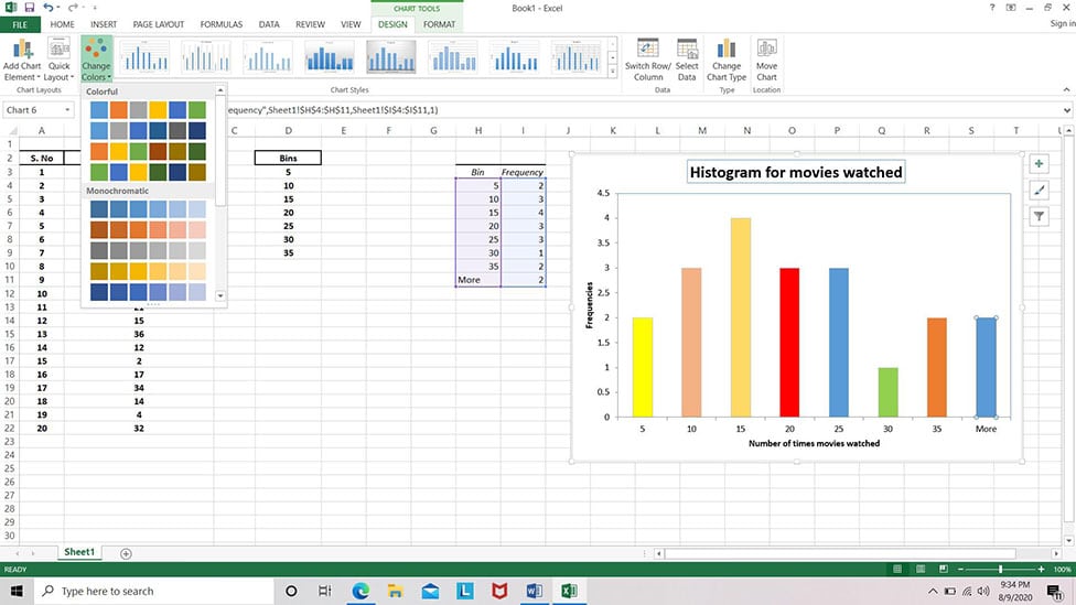
How to Create Histogram in Microsoft Excel? - My Chart Guide
How to Customize Your Excel Pivot Chart Data Labels - dummies The Data Labels command on the Design tab's Add Chart Element menu in Excel allows you to label data markers with values from your pivot table. When you click the command button, Excel displays a menu with commands corresponding to locations for the data labels: None, Center, Left, Right, Above, and Below. None signifies that no data labels should be added to the chart and Show signifies ...
components - What can I use to implement a doughnut chart in iOS ...
Add a DATA LABEL to ONE POINT on a chart in Excel Method — add one data label to a chart line Steps shown in the video above: Click on the chart line to add the data point to. All the data points will be highlighted. Click again on the single point that you want to add a data label to. Right-click and select ' Add data label ' This is the key step!
Excel Charts | Computer Technology
How to Create Line Charts in Excel (In Easy Steps) Use a scatter plot (XY chart) to show scientific XY data. To create a line chart, execute the following steps. 1. Select the range A1:D7. 2. On the Insert tab, in the Charts group, click the Line symbol. 3. Click Line with Markers. Note: only if you have numeric labels, empty cell A1 before you create the line chart.
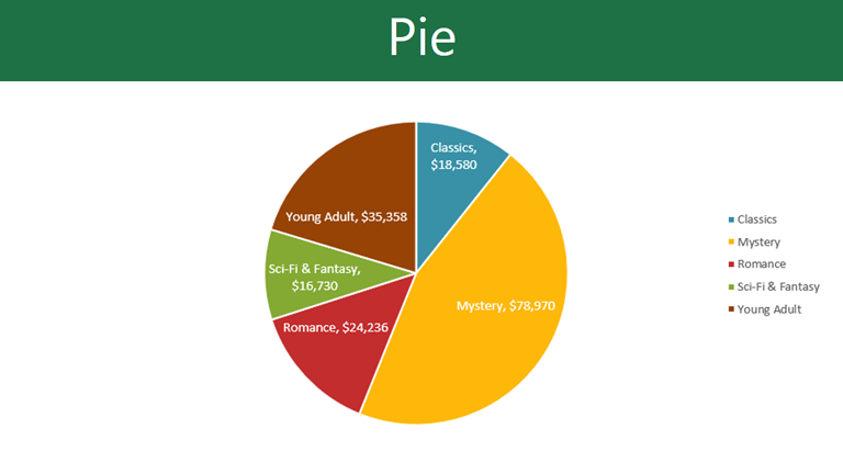
How to Make Pie Chart with Labels both Inside and Outside - ExcelNotes
Pie Chart in Excel | How to Create Pie Chart - EDUCBA Follow the below steps to create your first PIE CHART in Excel. Step 1: Do not select the data; rather, place a cursor outside the data and insert one PIE CHART. Go to the Insert tab and click on a PIE. Popular Course in this category
Graphing with Excel - BIOLOGY FOR LIFE
EXCEL 97 Charts: Column, Bar, Pie and Line Pie charts from this example, both the default Excel version and an improved version after some customizing, are given on page 3 of the pdf file Excel chart example output. LINE CHARTS. The line chart is not really helpful for these data. The line chart is best used for numerical data that are observed over time. .

CD: Pie of Pie Charts
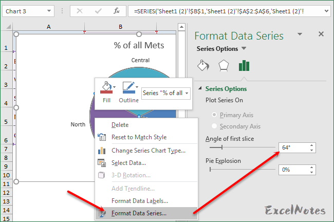
excel - Positioning data labels in pie chart - Stack Overflow Sub tester () Dim se As Series Set se = Totalt.ChartObjects ("Inosa gule").Chart.SeriesCollection ("Grøn pil") se.ApplyDataLabels With se.DataLabels .NumberFormat = "0,0 %" With .Format.Fill .ForeColor.RGB = RGB (255, 255, 255) .Transparency = 0.15 End With .Position = xlLabelPositionCenter End With End Sub
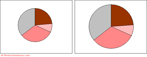
Excel Charts - Show Pie Charts in Proportion
How to display leader lines in pie chart in Excel? - ExtendOffice To display leader lines in pie chart, you just need to check an option then drag the labels out. 1. Click at the chart, and right click to select Format Data Labels from context menu. 2. In the popping Format Data Labels dialog/pane, check Show Leader Lines in the Label Options section. See screenshot: 3.
PIE chart labelling values with reference lines
Leader lines for Pie chart are appearing only when the data labels are ... It's only when they are moved, the leader lines are possibly needed because they are further from the point they are labeling. Best fit tries (as best Excel can) to arrange the labels without overlapping. It the wedges are large enough, the labels go inside, or Inside End.
How-to Add Label Leader Lines to an Excel Pie Chart - Excel Dashboard ...
excel - Prevent overlapping of data labels in pie chart - Stack Overflow However, the client insisted on a pie chart with data labels beside each slice (without legends as well) so I'm not sure what other solutions is there to "prevent overlap". Manually moving the labels wouldn't work as the values in the chart are dynamic. ... How to avoid data label in excel line chart overlap with other line/label? 0.
Post a Comment for "45 excel pie chart labels with lines"